This post was written in co-authorship with @Eleni Santorinaiou and @Elizabeth Antoine

Disclaimer. This article represents personal experience and understanding of the authors. Please use this for the reference only. This article doesn’t represent official position of Microsoft.

Simplicity is an ultimate sophistication.

— Leonardo Da Vinci

Before We Begin

In this article we are talking a lot about different methods of comparison and selection of databases. Also, we are presenting an alternative approach for looking and considering different options. At the same time, I would like to highlight that this is just one of the viewpoints. Please use below as a reference rather than a prescriptive guidance.

And may the force be with you.

SHOKING HAZARD! Equipment you might need before reading this article.

https://www.wired.com/2010/12/collectors-wonder-does-darth-vader-costume-borrow-from-19th-century-firefighters/

Important note: What is and What isn’t this Document

This Decision Tree is:

• Map of the Azure Data Services with the main goal to help you to navigate among them and understand their strengths and weaknesses.
• Supplementary material to the officially published Microsoft documentation helping you to define and shape your thought process around selection of the certain data technologies and using them together in your solutions.

This Decision Tree is not:

• A Definitive Guide to selection of Data Technologies.
• Business / politics related document. All the criteria we were using are purely technical.
• Not a pattern or use-case focused document.
• Not a competitive analysis of any kind.

We are keeping some responsibility on maintaining this document as long as we can but still would recommend verifying points in the document against Microsoft official guidance and documentation.

Also do not hesitate to apply common sense and, please check things before putting into production. Not all the situations are the same / similar.

The article has four chapters:

Chapter 1: Read and Write Profiles – explains the premise of the decision tree.

Chapter 2: Navigating Through the Decision Tree – guide to navigate through the decision tree.

Chapter 3: Mapping Use Case to the Decision Tree – examples of how the decision tree is used for different use cases.

Chapter 4: Getting Access and Providing Feedback – Finally, do not hesitate to provide us with your experience / feedback. We will cover how to do this in this chapter.

Chapter 1: Read and Write Profiles[1]

Our data technologies were developed mainly for two major purposes. And guess what, these are not encryption and obfuscation rather reading and writing data. Actually, mainly for reading as (and I hope you agree with me) there is no point in writing data you cannot read later on.

Surprisingly, we never compare data technologies based on their actual read and write behavior. Typically, while compare data technologies we are (pick all that applies):

• Focusing on some subset of the requirements.
• Checking “similar” cases.
• Adding technologies to the design one-by-one.
• Using “Reference Architectures” and “Patterns” in seeking for forsaken tribe knowledge.
• Surfing Internet long nights in a hope that by modifying the query we can find some kind of sense.

Basically, we craft design of our data estate based on experience, preferences, and beliefs. When our group faced first time the need to compare different technologies and recommend one, our first thought was – it is impossible. How would you compare NoSQL database to Ledger database?

Very simple – using their fundamental read and write goal as a foundation for such a comparison. The essence of the technology remains the same as well as a goal of its creation. A sheep cannot become a tiger ?

Well, in most of the cases ?

Picture: Paul Faith / PA (https://www.telegraph.co.uk/)

This beautiful “Tiger Sheep” won the first prize in the first ever sheep fashion show at Glenarm Castle in Northern Ireland, as part of the Dalriada Festival.

To give you an example, Apache Kafka was created to write tons of small items in sequential fashion and read them one-by-one (at-least-once delivery is a direct consequence of it). Does anyone use it for large-scale analytics on archival data? NO! The reason is simple – because of its read-and-write profile. These are widely known and defined by the industry (effectively, by all of us) and are used quite for some time.

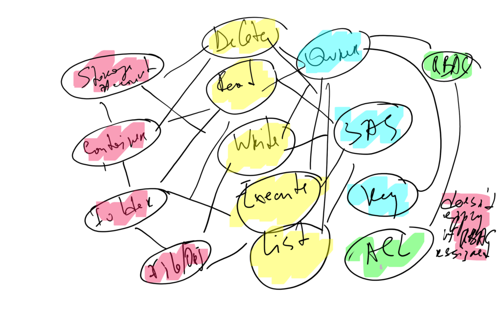
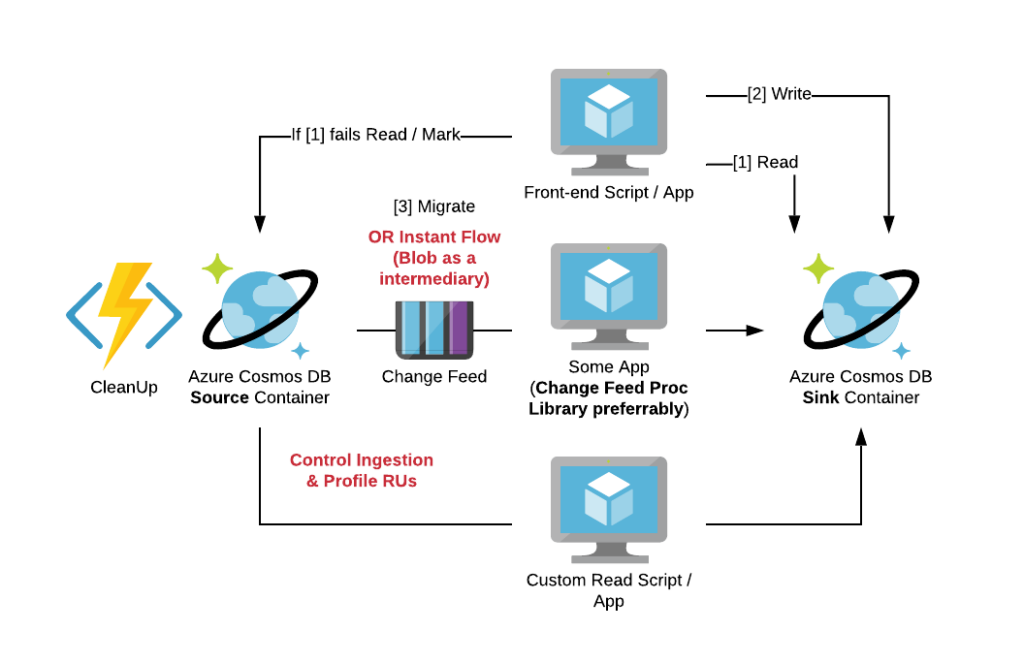
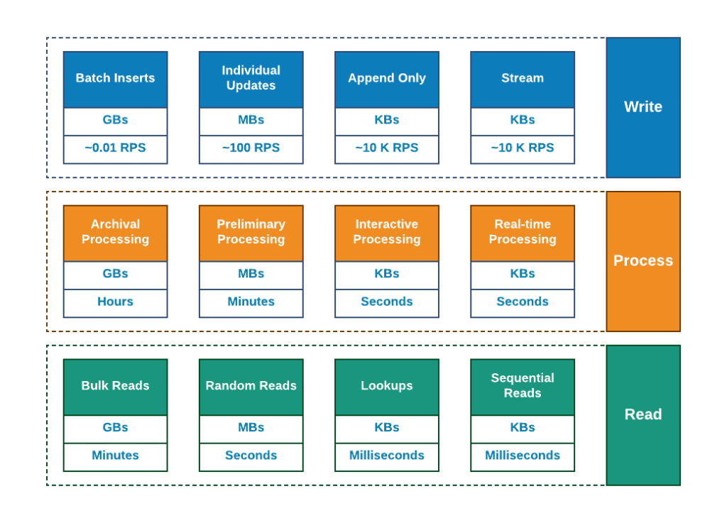
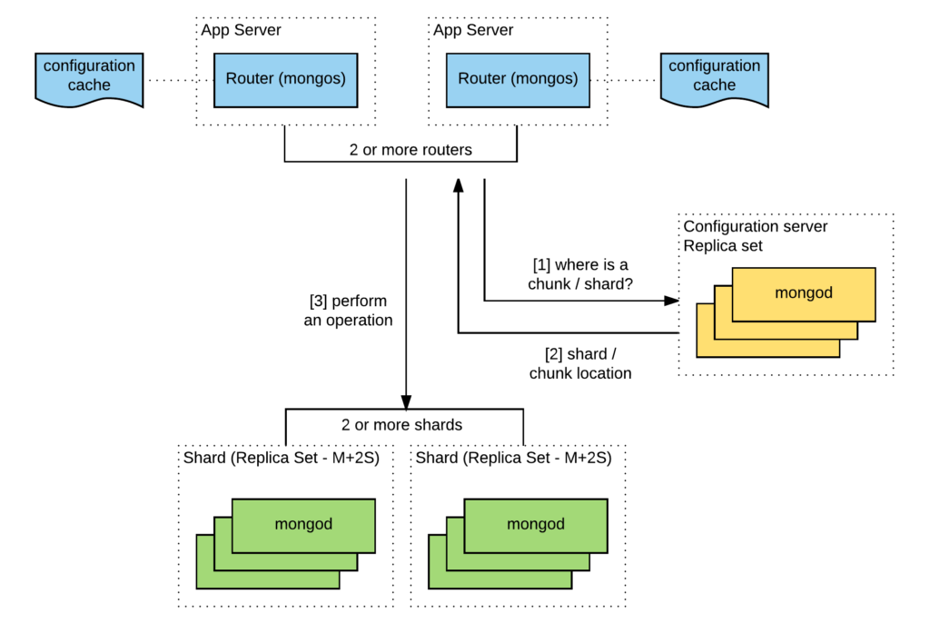
Let us take a look at the following diagram (I am borrowing this from one of the previous articles “Why so many databases?”).

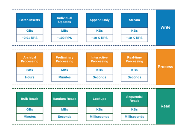
Intuitively (and, hopefully, obviously), if some data has a write path it should also have a read path and may or may not have one or more processing capabilities / tools / approaches.

Of course, loads of the technologies and vendors are claiming that one single solution can solve all the possible issues but the entire history of rise of Data Technologies over the last decade shows that it is surely not the case any longer.

Side Note: In fact, when some great technology emerges it always refers to the concept of “Purpose Built Technologies” while becoming more and more mature, it starts claiming to fit in virtually any use case possible.

Well it seems that we have finished with WHY and already started with WHAT? Let’s move on and show you one of these Decision Trees in more details.

Chapter 2: Navigating Through the Decision Tree

So, in order to help you to navigate across ever-changing and pretty complex Azure Data Landscape, we have built a set of decision trees based on the concept of read and write profiles. Conceptually Decision Tree looks very simple.

Well, it is not that simple obviously. The good thing is that it covers almost entire Azure Data Portfolio in one diagram (which is comprised of more than 20 services, tens of SKUs, integrations and important features). So, it just cannot be super simple. But we are trying ?

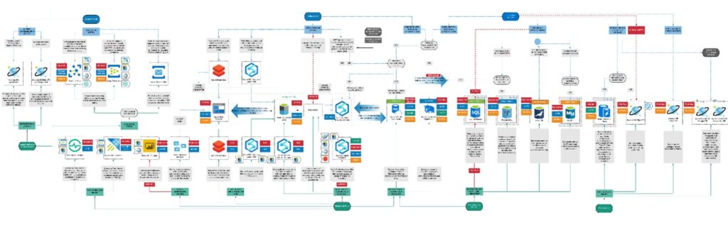
In order to guide you through it, let’s just paste a small example (subset) of this decision tree here and demonstrate you some of the main features and ways to navigate through them.

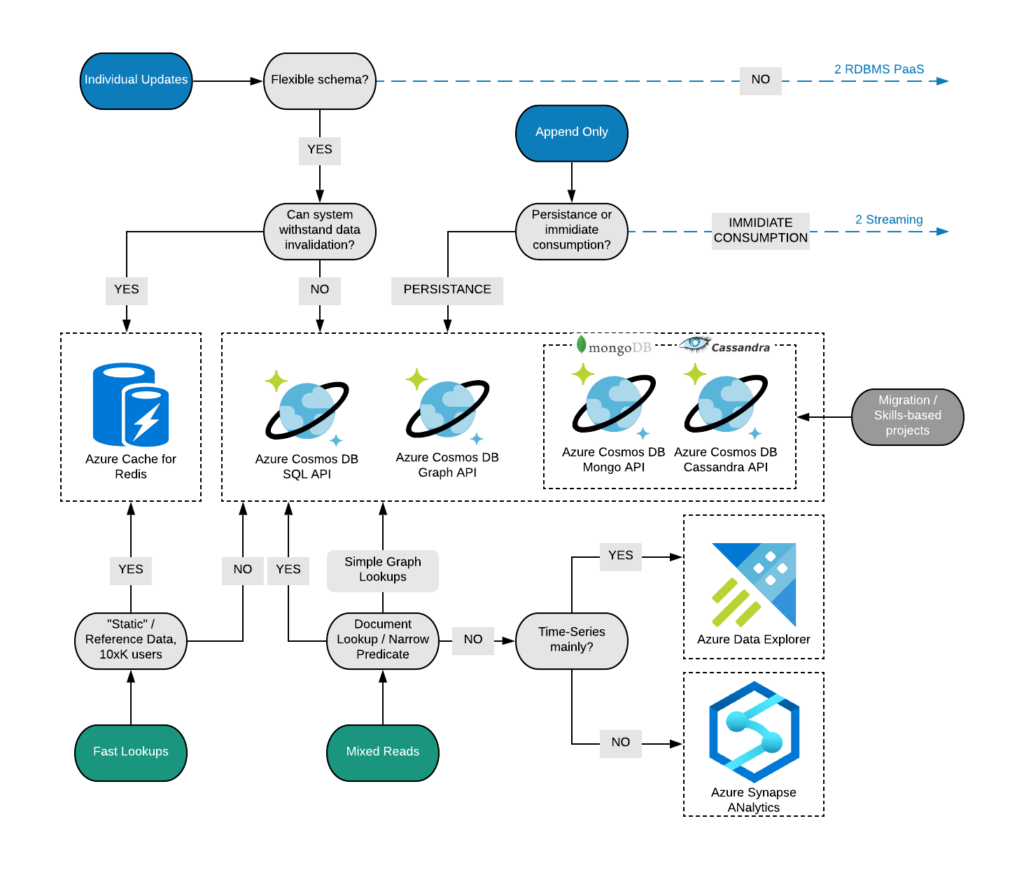
Basic Navigation

It is comprised of two main paths read and write patterns. Write pattern from top to the middle marked with blue boxes and lines and read pattern – from the bottom to the middle marked with greenish lines and boxes. This represents some of the fundamental differences in behavior of various technologies.

In the grey boxes you can see either questions or workload descriptions. As mentioned, this approach is not strictly defined in the mathematical sense rather follows industry practices and includes specific features and tech aspects which differentiate this technology from others.

In case of the doubt, just simply follow yes / no path. When you have to choose among descriptions, you have to find the one which fits best.

Below are the components of a simple navigation.

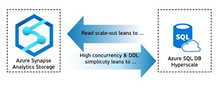
Leaning

There are also some more tricky parts, where you cannot say with certainty which workload will be a better fit. In such cases we are using wide blue arrows representing “leaning” concept. Pretty much like in one of the examples below.

There is one more style of “leaning” which is represented by the so-called “paradigm”. In some cases there are technologies which will be preferred when you are using particular programming language or stack. In our decision tree this is represented by the notion of “paradigm” as described on a picture below.

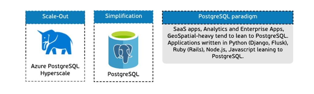
Typically, in one paradigm we have more than one product available. To distinguish the main goal of the product within certain paradigm we are using some code wording like in the example above. This goal is represented by one word which is shown above the box with the service and holds the same color as a paradigm.

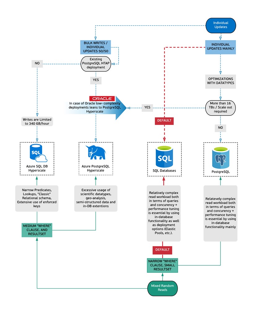
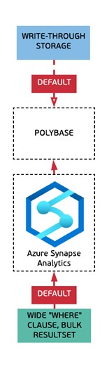
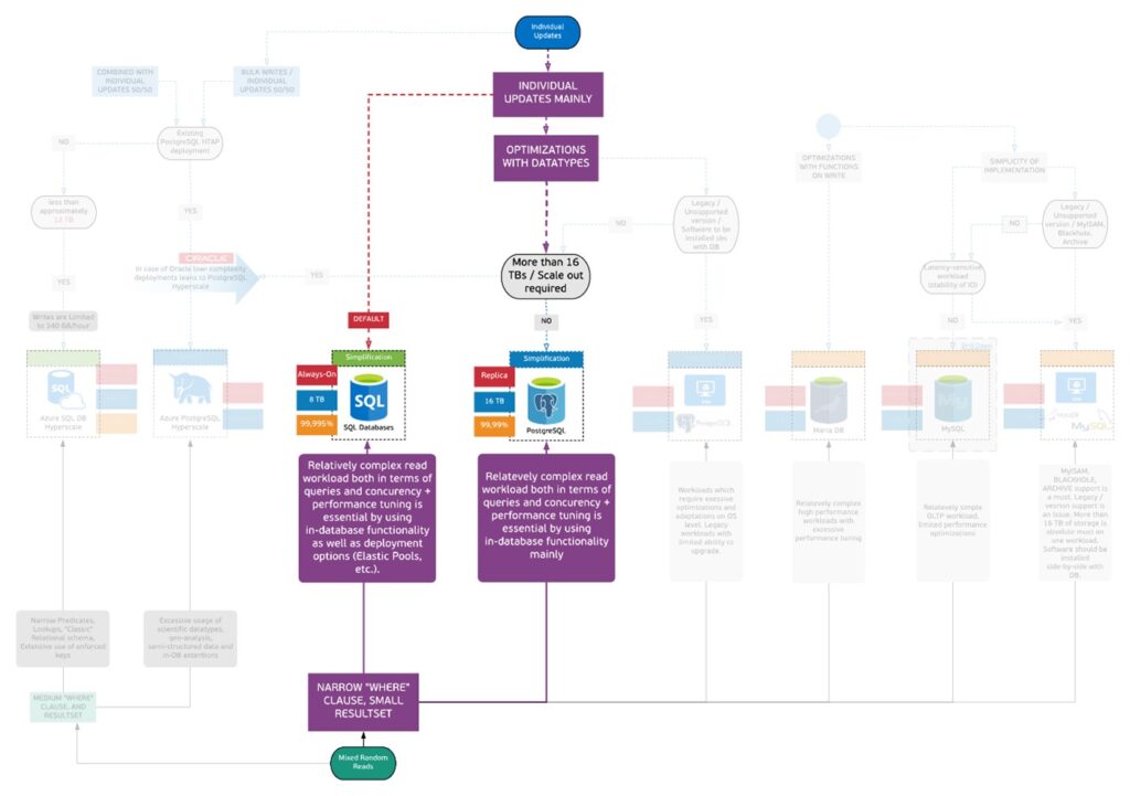
Default Path

In most of the technology patterns we also have a “default” path for reads and writes. Typically for a greenfield project this is the easiest and richest path (in terms of functionality, new features and, possibly, overall happiness of the users).

Drill Down

In some cases, we also have implemented a drill-down approach to simplify the navigation. Drill downs lead to a different diagram explaining some details around service offerings or SKUs for a particular product / service.

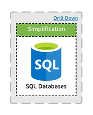
Drill down will bring you to the new Decision Tree which is specific for the particular technology (such as SQL Database on Azure, PostgreSQL or others). These Decision Trees are following same / similar patterns with some reduced number of possible read and write profiles (as shown on a diagram below). On these Decision Trees SLAs, High-Availability options as well as Storage and RAM limits are defined on the per SKU basis.

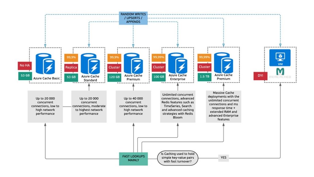
SLAs & Limitations

Another cool feature of the Decision Tree is a depiction of maximum achievable SLA, High Availability options and Storage / RAM limits (when it makes sense).

These are implemented as shown below. Please remember that these might be different from SKU to SKU and only the maximum achievable is shown on the main Decision Tree.

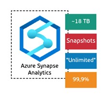
Please note that all / most (just in case we forgot something) of the icons with limitations, HA & SLA are clickable so you will be redirected to the official Microsoft documentation.

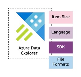
Developer View

One of the newest features is a Developer View. In this view we are listing all the Procedural Languages supported by the technology as well as SDKs and some important limitations of size of items or resultsets where applicable. Also we are depicting supported file types and formats.

We are planning to make these references to the official Microsoft documentation (pretty much like it was done with SLAs, Storage, etc.)

Read and Write Profiles Do Not Match

With two separate profiles for reads and writes there is a very important and frequently asked question: “What if read and write profiles do not match?”

Let’s answer with the question. What do you typically do when your technology used for writes is not suitable for doing reads with the pattern / functionality required? The answer is quite obvious – you will introduce one more technology to your solution.

To help you to find which components can be directly integrated with each other we have introduced the concepts of “Integration In” and “Integration Out”. The example of the notation is shown below.

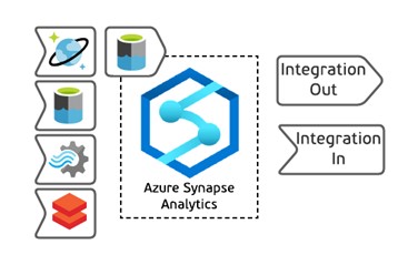
In this example we can see that Azure Synapse Analytics can accept data from:

• Azure Cosmos DB using Azure Synapse Link
• Azure Data Lake Store Gen2 / Blob Storage using CTAS functionality of Polybase
• Azure Stream Analytics via output directly
• Azure Databricks using Azure Databricks Connector for Azure Synapse

And export data through ADLS Gen2 using CETAS statements of Polybase.

As you may see on the Decision Tree itself, we can only see that such an integration is possible, but we are not specifying exact mechanism or its limitations. If you click on this icon, you will be redirected to the official Microsoft documentation.

One more important note here. We do not show Azure Data Factory on this diagram as this is the service which meant to be used across the entire Azure portfolio and adding it to the diagram will make it even more messy. So, we implicitly mean that Azure Data Factory can be used to integrate with most of the services mentioned on the Decision Tree.

Ok, let’s take a look on how to apply this in practice. In the next chapter we will cover some examples of using Decision Tree to craft the architecture and select appropriate technology for your workload.

Chapter 3: Mapping Use Case to the Decision Tree

Why and How to Map Your Use Case to the Decision Tree

As you can see, these Decision Trees can be pretty complex but at the same time they represent almost full subset of data technologies. At the same time, industrial and technological use cases might still be very relevant especially if combined with the Decision Tree as a frame for discussion.

In such case one can clearly see not only choices made but also choices omitted. Also, it can immediately give you an idea which alternatives and when you may consider.

HOW? Just shade out all what is not needed and add your relevant metrics for the decisions made (for instance, predicted throughput, data size, latency, etc.)

Let’s take a closer look on how we can do it. And we will start with a small example.

Use Case: Relational OLTP / HTAP

In this example, your business specializes in the retail industry and you’re building a retail management system to track the inventory of the products in each store. You also want to add some basic reporting capabilities based on the geospatial data from the stores. To decide what is the best database for these requirements let’s take our uber tree and start from a write pattern.

• The data for the orders, users and products get stored as soon as it arrives, and it gets updated in an individual basis. The throughput of such system is not high.
• The schema of the entities is expected to be the same and a normalized logic is preferred to make the updates simpler.
• Your store needs to support geospatial data and indexing

This already narrows down our choices in the RDBMS space. Moving to read profile.

• The queries will have different levels of complexity, a user might need to get the stock of a specific item in a single store, or even join the data from stores that are located to a distance close to a specific store.
• The store manager will need to have a report available that it will show which days and time most traffic is expected.
• HQ will need to identify the positive or negative factors that have effect on a zip code’s total sales to increase the sales coming from the retail channel.

Since the queries have some geo-related clauses Postgres could be a good candidate and since some analysis and visualization is required SQL would be another option. Going further down, you could discuss with the development team the application stack and more specifically the programming language. If the app is written in node.js or Ruby, Postgres will be a great choice, otherwise, with .net Azure SQL will be the perfect solution. Other factors to take into consideration would be the amount of data to be stored, how to scale out if the data increases and the HA SLAs.

Use Case: Mixing the write and read patterns

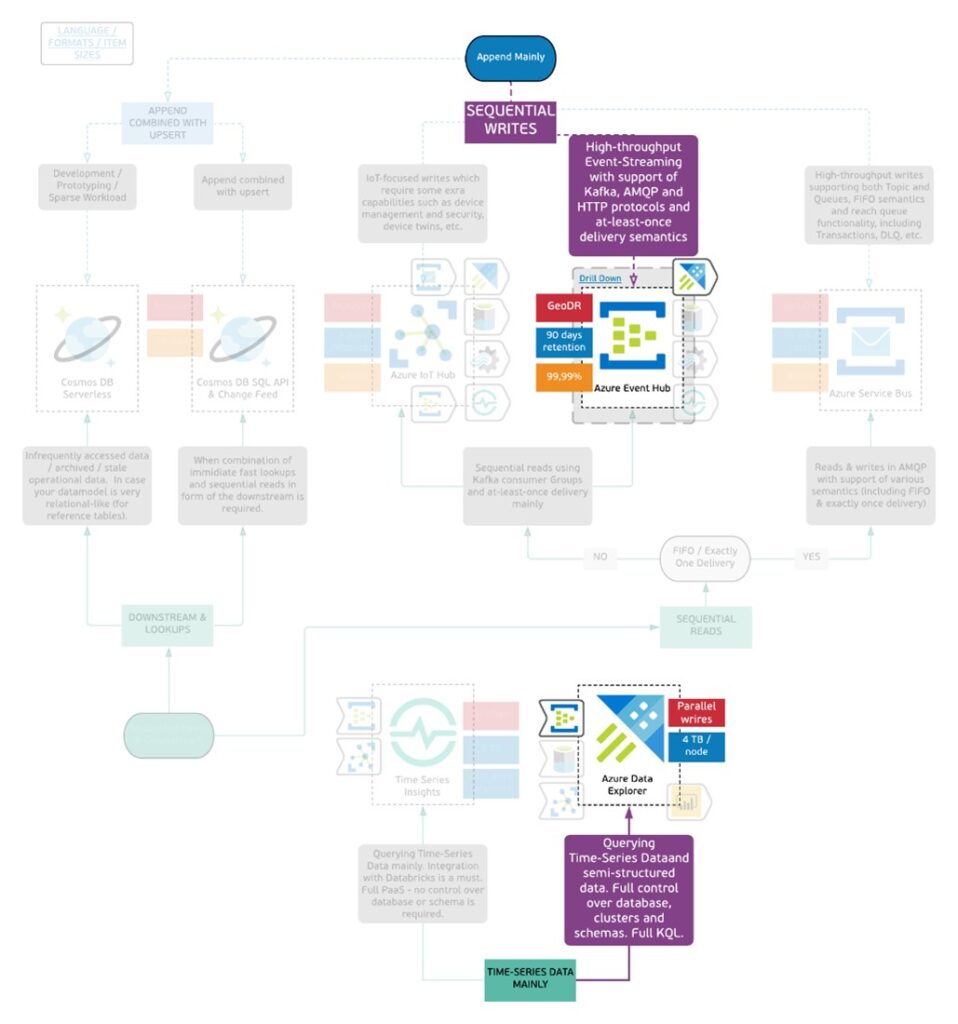
The next example of how the Uber Tree can be used as a tool to produce a data architecture comes from the gaming space. Your team is building new features for a massively multiplayer online game and they need to collect and store all actions of the players, analyze those that matter in near-real time and archive the history.  As usual, we will start from the write profile.

• The events are captured and stored and are never updated.
• High throughput is expected with hundreds of thousands of events per second.

For the specific use case seems that there is a single path for the writes; Event Hub answers those requirements. But the way we will process and read the data is not in a sequential order. More specifically:

• The data needs to be read in a time-series manner prioritizing the most recent and aggregating based on time.
• Need to narrow down the analysis to the metrics that are relevant for a particular game and also enrich the data with data coming from different sources, so basically, you need control over the schema.

On the read pattern, it looks like Azure Data Explorer would be the most suitable store.

In this case, where two different profiles for the write and read are identified, we will leverage two solutions that are integrated. Azure Data Explorer natively supports ingestion from Event Hub. So, we can provide a queue interface to the event producer and an analytical interface to the team that will run the analysis on those events.

Use Case: Analytics

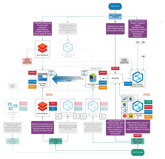
In this example, your business specializes in the energy industry and you’re building a analytics platform for power plant operation and asset management. It would include all the necessary pieces, from condition monitoring and performance management to maintenance planning, risk management and market scheduling. To decide what is the best approach for these requirements let’s start with the write patterns of our uber tree.

• Since operating a power plant generates a large amount of varying data, the platform must have the ability to process batch data coming in huge volumes.
• 70% of the data is structured.
• The data coming from meters need to be processed near real time and involves complex processing before it can be unified with the data from performance, risk, and finance systems.

This already narrows down our choices to Azure Synapse and Azure Databricks with combination of Azure Storage & ADLS Gen2 with Polybase

 Moving to read profile.

• The queries will have different levels of complexity,
• Takes the data and information from the source systems, merges them to create the unified view to make it possible to monitor the performance of the plants/assets through an executive dashboard.
• Machine learning to provide decision support.

Since the requirement is to unify the huge volumes of data across different source systems where 70% of the data is structured, PolyBase would be right choice to land the data in Azure Synapse Storage and perform the transformations using Synapse SQL to create the dimensional model for historical analysis and dashboarding. There is also 30% of the unstructured data that needs to be processed before merging that into the dimensional model where optimized spark engine like Databricks is a perfect fit for purpose and also can be extended to the ML use-cases for decision support. Other factors to take into consideration would be the amount of data to be stored, how to scale out if the data increases and the HA SLAs.

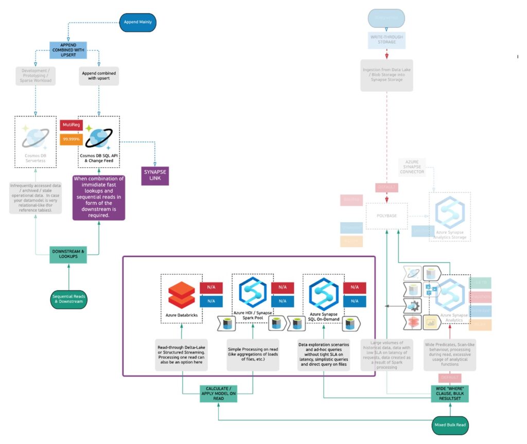
Use Case: HTAP

In this example, your business specializes in the healthcare industry and you’re building a platform for patient outreach and engagement. You are trying to build an advanced analytics solution looking to take chronically unwell patients that have high utilization of emergency department/ unplanned inpatient services and, through a more coordinated provision of ambulatory services keep them well at home. To decide what is the best approach for these requirements let’s start with the write patterns of our uber tree.

• The write pattern itself is largely event-driven and completely serverless, which aggregates messages from close to 200 data sources across the organization.
• They also have a million different EHRs and other sources of data (Radiology, Cardiology, Surgery, Labs Systems, etc.) and also millions of transactions per day.
• Have laws requiring data for each patient to be kept for at least 7 years (28 years for newborns).

This already narrows down our choices to Azure Cosmos DB for capturing the patient data across the different systems and to decide on the ability to build the analytics solution on the data captured in  cosmos DB, we now look at the read profile.

• Real time data must be available as soon as the data is Input, updated or calculated within the Cosmos DB database.
• Complex analytical queries must report results within 900 seconds.

Since the requirement is to provide the ability to do advanced analytics on the data captured in Cosmos DB but in near real time, the ETL approach cannot be leveraged here. The Synapse Link in Azure Synapse Analytics or Databricks could be considered as the possible options. If the usage pattern is ad-hoc or intermittent, you may gain considerable savings by actually using a Synapse Link solution compared to a cluster-based solution. This is because the SQL On-Demand will be charged per data processed and not per time that the cluster is up and running, hence you wouldn’t be paying for times when the cluster is idle or over-provisioned.

Chapter 4: Getting Access and Providing Feedback

Here we are. Thank you for being with us up to this moment. This will be the shortest Chapter – we promise ?

You can find interactive Decision Tree on GitHub Pages by following this link: http://albero.cloud/

All the materials can be found in a public GitHub Repository here: https://github.com/albero-azure/albero

You can provide your feedback / submit questions and propose materials via Issues of the GitHub Repository.

Thank you and have a very pleasant day!

BTW. Just tested it from my smartphone and it also looks pretty nice ?

---

[1] In one of scientific works (still in review and will be published soon) Andrei Zaichikov is proposing a formal definition of read and write profiles in form of quantifiable random numeric vectors and scales. It is not used in this work.

Disclaimer. Services are changing – please always check with the official Microsoft documentation before applying in practice.

Recently I was asked by several customers to explain the authentication features of Azure Data Lake Storage Gen2 and how they are used together. Honestly speaking I was a bit puzzled. “Everything should be in the documentation. It should be obvious” – I thought for myself.

But when I was trying to compile something from existing materials I have suddenly discovered that it might be a bit confusing and requires some time just to get through all the options. So, I have created a short diagram.

Sorry wrong diagram – the real one below.

Just to recap very quickly.

The authentication against ADLS Gen2 can be done with or without identity. The rights can be granted on several levels of the resource hierarchy and different methods have different granularity of permissions. Permissions may or may not have inheritance. As simple as that.

And remember you can always refer to the official documentation which is much more detailed. Also follow the updates here. In case some functionality is missing please feel free to vote / propose it here.

Have a nice and productive week!

Disclaimer. All the opinions and recommendations are my own. Do not believe in words only – test and adjust to your case.

Today we have loads 0f different technologies, hard to believe that anyone can be Expert in some of these. But I do believe that occasionally you need to get quickly a short but deep overview of what the certain technology is about.

Here is the algo I have started using some years ago and improved over the last five years working for Microsoft and Amazon. It allows me to dig out important information about the technology at a very high speed and get a sense of how, why and when it can or cannot be used.

So (for data technologies):

1. Start with the read and write path – how the data is being written and read. What temporary structures are used and where they are located, which timeouts can be set, what additional operations are being performed during the process etc.
2. Check technology limitations – functional limitations and deployment limitations. Try to find both official and non-official limitations.
3. Search for known performance issues – in which workloads it was discovered, how these issues were eliminated. Look through performance optimization best practices – it will give you a good overview of the best and the worst case scenarios of usage.
4. Watch how it fails – ideally postmortems from the customers. It will provide you with a good idea of flaws in the High-Availability and Disaster Recovery behind the marketing curtains. Also, it highlights limits of scaling.
5. Do a small research on the ways how it interacts with other technologies or system components – not everything is possible by default. You may discover some missing integrations, driver deficiencies, etc.

Applying this approach from time to time will build you muscle memory so the entire process can take around an hour or two. In addition to the five points above I would also recommend to try the tech out. Here I am typically working with the CLI-style experience as it helps to unfold some hidden things.

Of course, it doesn’t substitute the real methods of learning and works just as an emergency toolbox for getting acquainted with the technology you have never touched before or haven’t been working with for years.

Hi All

Just a short note on Azure Synapse. Over the last couple of months, we witnessed several major announcements and service renamings so you may be confused on what exactly Azure Synapse is and what components are included.

Please use this small graphics I have crafted. In case you would like to try Azure Synapse Workspaces, please use our great Quick Start tutorial here.

Some links to the functionality mentioned.

• Azure Synapse Workspace
• Azure Synapse Workspace (SQL Pool)
• Azure Synapse Workspace (Spark Pool)
• Azure Synapse Link for Azure Cosmos DB (some extra info)

Have fun!

Disclaimer. This article describes findings when working with SSMA version 8.5 on one large PoC. The results in your environment might be different. In case you are relying on the estimates provided below, treat them as reference only.

In this short article I will briefly describe some of the findings from a large-scale PoC we were working on recently. This includes what was successful and what was not, a few time estimations and certain problems we faced using the tool.

The PoC included migration / assessment of ~10 000 tables and ~40 000 views from Oracle to Azure Synapse Analytics. The overall dataset size was ~ 10 TBs.

Our initial plan was to use SSMA for Oracle to migrate DDLs and long-tale data from Oracle and use spool offloading and Polybase to load data into Azure Synapse for the large tables. This plan was partially implemented and partially changed over the course of the PoC.

The process of working with SSMA for Oracle is:

1. Create an SSMA project. Please do not forget to give your project a meaningful name as it cannot be renamed later. When creating the project, please select the proper target (in our case it is Azure Synapse Analytics or former name of Azure SQL Datawarehouse).
2. Connecting to Source (Oracle). I started with applying Oracle Data Pump packages (DDL only) to one of my test Oracle instances. After that I used this instance for the initial (test) conversion.

Note. Please refer to SSMA docs for a current set of permissions required for SSMA to run.

Recommendation. This is not possible to repoint the migration project to another source / target instance. You will have to start all over again. Reading metadata from Oracle was one of the longest processes (it took us around 24 hours to read the metadata for ~8000 tables and ~22000 views) so it is recommended to start the conversion with the real source database (we have to read metadata only once per project). Note. Conversion from production DB was 30% more effective than from imported Oracle DB.

Recommendation. When selecting the schemas, try to group these schemas in several projects evenly in terms of number of objects to transform and data to migrate. This will allow you to work on several parallel loads.

Note. All the actions described below are triggered with the action buttons from toolbar menu. The scope for the action is defined by selecting the objects in the tree view (Metadata Explorer) to your left. You may need to select some specific objects out of thousands so you will find “Advanced Object Selection” functionality very useful. Just use this small button ?

Note. Reading metadata from Oracle doesn’t have any progress bar.

• Connecting to Target (Synapse). Please check that you can connect from SSMA host to Synapse before starting the connection Wizard (it will simplify the connection troubleshooting). Please refer to Synapse Docs to check how to connect to your Synapse Analytics instance.

Recommendation. We recommend to use the smallest DW at this stage (DW100) to avoid high costs as size of the DW and resource class has no impact on DDLs conversion / application performance.

Recommendation. When creating Azure DW users, keep in mind the following. Workload classes will be assigned to users. If you are planning to run the SSMA projects for Data migration later on, you need to create as many users as parallel loads later on and assign proper resource class as per Synapse Documentation. Note. In our case I have created an xl resource class user which later affected our ability to execute parallel SSMA projects for data load.

Recommendation. Before performing any further actions, I recommend tweaking a couple of parameters on SSMA side. First is to go to Tools->Global Settings->Logging and set up all the Logging to Debug mode. It may help you and support teams later. Second, open Tools->Project Settings->Synchronization and redefine Query Timeout (in case doing assessment in parallel with something else, I use 100 as a default). This will keep you safe from timeouts in most of the cases.

• Reading metadata from Oracle. You can select the schemas for which the migration should be performed. This will trigger the metadata reading process which takes a while. Reference point for me is around 15 minutes per 100 tables.
• Creating the Migration report. You can create an html-based migration report with all the migration efforts estimated and mitigation actions listed.

Note. In my environments this report was fully shown only in Microsoft Edge browser. In all other browsers most of the valuable information was not displayed. However, please also note that I did not spend much time trying to fix this.

Report produces two main views.

• Statistics View (How many objects / components were migrated)
• Code View (How particular object was converted on the code level)

Note. Reports are stored within the SSMA Projects/[ProjectName]/report/report[date-time]. Use mainindex.html to access the report.

• Convert Schema. This action transforms the DDLs and code ignoring exceptions highlighted in the report to the target (in our case Azure Synapse). Please note that this action will not apply the changes to the target – only saving it within a scope of the project.

Note. This action typically takes some time depending on the size of the scope selected. In the worst case ~8000 tables and ~20000 views it took around 36 hours to do all the conversions. We benefit from splitting the work in several parallel projects (on different schemas to avoid inconsistency in the project status). Conversion for 100 tables took me ~20 minutes.

• Apply Schema. To apply schema to the target, just right click on the target DB and select Synchronize with Database. This will call a pop-up windows with summary of all the changes to be performed on the database.

This operation is faster than previous ones but still takes roughly 10-15 minutes per 100 tables and on the large scale also takes up to 12-18 hours on 8000 tables / 20000 views.

Note. If you already have some ideas on how the distribution will look like in Azure Synapse, you can use SSMA to define the distribution style. To do that please use the following tab.

• Migrate Data. SSMA can perform data migration using the direct read from Oracle. It will take care of data types conversion, batching and writing to Azure Synapse.

Note. In my case I was able to migrate 7 GB table in 15 minutes. At the same time due to the different reasons we experienced high error rate (~10% of tables were not able to migrate). In one of the threads we were able to migrate ~800 tables in 12 hours. The overall size of this dataset was close to 400 GB.

Note. To track the migration status, use Data Migration Error log (location can be found in Tools-> Global Settings->Logging.

In case of using SSMA the project ends up here. However, in our case we were required to do several more hands-on things:

• Offload and migrate large tables. For this we used a generator based on the functionality of COPY INTO command (you may face some of the issues with customer UTF characters as delimiters) and EXTERNAL TABLES.
• Perform manual changes in SQL code and apply them to DW. This was major hands-on activity
• Perform testing.

As you can imagine two last points are the most complex ones ? where you may need to allocate most of the time and efforts. This is a very vast topic and please refer to Azure Data Migration Guide for further information.

In conclusion, SSMA for Oracle is a great tool with tons of functionality which alone can be used for small and medium migrations within reasonable time frame. It also should be considered as one of the key tools in the toolbox for large DB migrations.

Stay safe and have a great day!

Hi there

I was always wondering – why we have so many different databases. If you take a look at raking published on https://db-engines.com/, you will easily find out that there are 334 database technologies.

The question is if we need that many and why people are using that many databases. I know that it is a complex question and there are various different viewpoints on it – historical, cultural, technological, etc.

Let me describe how I see it from purely technical viewpoint.

We have numerous different types of the database-related workloads. Typically, what we do in the database is read, write and process (in most cases). These processes are different by nature and we do care about different parameters of each process. Also, as you may imagine, database exists in some environment and not always we can or want to influence or change it. So, we have a combination of database and environment it exists in.

If we classify three major processes we have in the database and will add some main parameters we do care about to the single chart, we will have some initial idea from where this variability comes from.

Indeed, this is a simple and self-evident, right? We do have many types of the technologies (like MPP, HTAP, OLTP, Cache, Stream, etc.) to accommodate different read and write patterns.

This diagram also can illustrate the reason behind the rise of polyglot persistence. If you have streaming as a write path and then consuming data in large batches there will be, most probably several major technologies and these will be decoupled one from another. At the same time if you are processing time, required read latency and write throughput are within the same pattern probably you will end up using one single database technology for most of your needs.

That‘s interesting but the one thing that this approach doesn’t explain is why we have hundreds on them (even if we put development fashion and personal preferences aside). In order to explain this we will need one more graph.

Apart from the workload, environment and their parameters we are also looking on the several main things (even if we are not doing it from the start we will be considering them soon after the real works begins), such as:

• Deployment Options – for example, hybrid deployments, mobile deployments, deployments on specific hardware as well as possible deployment optimizations. This also includes HA & DR, maintenance routines, etc.
• Possible Optimizations – most of the existing databases were born when developers faced new or unique challenge, so those technologies were adapted for solving very narrow cases. For instance, CouchDB is very good in supporting replications of various styles, SQL Lite works on cell phones and Aerospike is extremely efficient when it comes to in-memory processing. Even in Caching (which is very narrow) people are using Memcached for working with small Key-Value pairs (very efficient when it comes to RAM) while using Redis for more complex scenarios.
• Cost implications – licensing, hardware, ability to scale and optimize cost based on various techniques.

Combining these two graphs together will give us a pretty good (but for sure even not close to full) picture on why we still have so many database technologies.

Choose wisely 😉

Original blog post was written by me and published in AWS Database blog.

In this blog post, I will share experiences from a cross-regional migration of large-scale NoSQL database clusters (from Europe to the U.S.). The migration was a joint project implemented by the Ops team of our reference customer, FunCorp, and AWS Solutions Architects.

“Our flagship product, iFunny, is one of the most popular entertaining apps for American youth,” said Roman Skvazh, CTO of FunCorp. “For the last five years, the service has gained a considerable audience. Our mobile apps are utilized by more than 3.5 million active users per day and are operated in all time zones. A back end of the app is implemented on Amazon Web Services and its scope is impressive.”

What Should We Migrate?

The iFunny product uses the following database services running on AWS:

• Apache Cassandra cluster – 25 nodes, 18 TB of data
• Apache Cassandra cluster – 18 nodes, 16 TB of data
• MongoDB cluster – 5 TB of data, distributed across 8 shards, each shard – replica set includes the master and two slaves
• MongoDB cluster– 150 GB of data, distributed across 4 shards, each shard – replica set includes the master and two slaves
• Elasticsearch cluster – search index of 1 TB
• Redis – one master and two slaves, with 15 GB, 10 GB, and 1 GB of data and very high write speeds

“Through the efforts of our DevOps and Back End teams, and together with AWS SA, we were to move all of our infrastructure from one AWS region to another with no downtime and no major changes in the application.”

Why Should We Migrate?

If you’ve ever asked yourself the question, “Why migrate everything?” consider FunCorp’s reason: In the beginning, FunCorp selected an AWS region based on the Russian market, but the iFunny app quickly gained enormous popularity in the United States. Up to a certain point, it was convenient to have a backend located on a different continent. However, the high networking latency began to affect the user experience. For this reason, a migration became one of the integral parts of FunCorp’s global UX improvement program.

FunCorp had some constraints and conditions:

• Zero downtime
• No changes in the application and database structure
• Minimal use of third-party tools

How Should We Migrate?
At first, we planned to implement the migration project using own capabilities for geo-distributed replication for each mentioned database (Cassandra, MongoDB, Amazon ElasticSearch Service, and Redis), but we faced several significant problems unique to each database.

MongoDB

The first issue had to do with mongos for MongoDB Shard, a routing service for shard configurations. The replication between the European cluster and the USA cluster ran smoothly and was implemented by using the standard features of MongoDB, but after switching the users to a new back-end MongoDB, the performance of mongos in the U.S. decreased considerably. The problem was that a geo-distributed cluster of MongoDB supported only one set of configuration servers, which were located in Europe at the time. The following diagram illustrates the initial setup.

Mongos had to call the configuration servers, which were located overseas, for virtually every operation. The good news is that mongos keeps its configuration cached. However, it’s not possible to increase the number of chunks or to reorganize the data between them by relying only on caches and without connecting to the configuration servers. Therefore, the server migration should have been done quickly.

The final migration algorithm looked like this:

• We created some instances in the target region beforehand, with a configuration identical to the current one, and then we incorporated them into the existing replica set of the initial clusters. Then we waited until the end of the data replication.
• Just before the start of the migration process, we switched off mongos balancing. Thus, the mongos processes in the target region used a cached version of the configuration.
• During the migration, we moved away all of the instances with the data in the source region, one by one.
• In the replica set, there were only instances in the target region left, and new primary servers were elected from among these.
• Finally, we migrated the replica set configuration to the new region.

Cassandra

To migrate the Cassandra clusters, we created an additional Cassandra data center in a Cassandra geo-distributed cluster with a standard EC2Snitch in the target region and connected them to existing clusters through a software VPN tunnel. After that, we started the nodes and began the replication process. The VPN tunnel was essential, because it allowed us to enable interactions between geo-distributed clusters without having to change the snitch from EC2Snitch to EC2MultiRegionalSnitch. In our case, that meant not only a change of the snitch itself, but also manual cluster scaling, support for address lists in security groups, interaction between nodes on a public IP, and many other things. We thought most of the problems were solved.

Unfortunately, just after we started the replication process, the performance of the original Cassandra cluster dropped significantly.

The problem was that Cassandra started replicating data to the new DC simultaneously, from all of the nodes in the source region to all of the nodes in the destination region, with respect to our replication factor and level of consistency. To solve the problem of performance degradation, we stopped the clusters’ replication processes and started rebuilding the nodes of the target cluster, piece by piece, two to three nodes at a time.

By taking this approach, we replicated both clusters without interrupting the work process and with almost no significant performance degradation.

After the replication process was complete, we were able to repair all of the nodes in the target cluster. After that, we switched the applications from the source DC to the new DC. Finally, we excluded the source DC from the cluster, and then terminated that DC.

Redis

We took a similar approach for the Redis migration. We created some new clusters, connected them to the existing one in the source region, and then started replication. The volume of data to be migrated was not a factor, but the data was changing at a very high speed. As a result, the data failed to be replicated within the time defined by the cluster replication window, and all of the data in the target cluster was invalidated.

After several weeks of research, we found a very simple solution to this problem with Redis replication. We created an SSH tunnel with compression and with ports forwarded to localhost:

ssh -C -L 6280:localhost:6379 $MASTER_REDIS

Next, we told the slaves to synchronize with localhost instead of the master:

redis-cli slaveof localhost:6280

Done! Now the Redis replication was running successfully. Because of compression, the replication lag did not increase and never approached a critical threshold in the replication window.

ElasticSearch
Our initial plan was to avoid the migration of the ElasticSearch search index and to instead re-create it in the destination region. Unfortunately, the procedure of index creation was too complicated. It required engagement from our development teams, which was outside the constraints and conditions of the project.

Fortunately, we found a perfect ElasticSearch plugin that allowed us to do backups, including incremental backups. You can find a version of the plugin here. (To find the right version, see the README.md.)

The use of the plugin greatly simplified the migration by:

• Creating an ElasticSearch cluster in a destination region.
• Creating an Amazon S3 bucket, with versioning and cross-region replication enabled.
• Creating a snapshot of the main data set and writing it to S3. The snapshot was transferred to the new region automatically.
• Restoring data from the snapshot in the target region.
• Repeating the preceding steps for the incremental backups. (In our case, the process of applying the incremental backups took 12 minutes.)

The results of the project
The project was successfully implemented and the back-end migration reduced latency by at least 40% for end-users when accessing the iFunny mobile back-end API.

However, it took us more than two months of experimenting and a month and a half for an actual migration.

Conclusion
Any database migration is a complex process. Ambiguous situations, such as the non-standard behavior of a database engines or a process that places a significant impact on the network, can always occur.

The best and safest way to migrate, free of data loss or similar surprises, is to test with real data and real configurations – and only afterward, to proceed with transferring the production database to a new location. Even if your application is not cloud-native, the use of cloud services allows you to experiment and to reproduce the existing use case in a geographically distributed environment, at real scale of clusters and data.

Hello and welcome to my blog. All the materials and content in this blog are based on my personal experience and do not reflect an official position of my current or former employers. For official recommendations, please refer to corresponding resources.